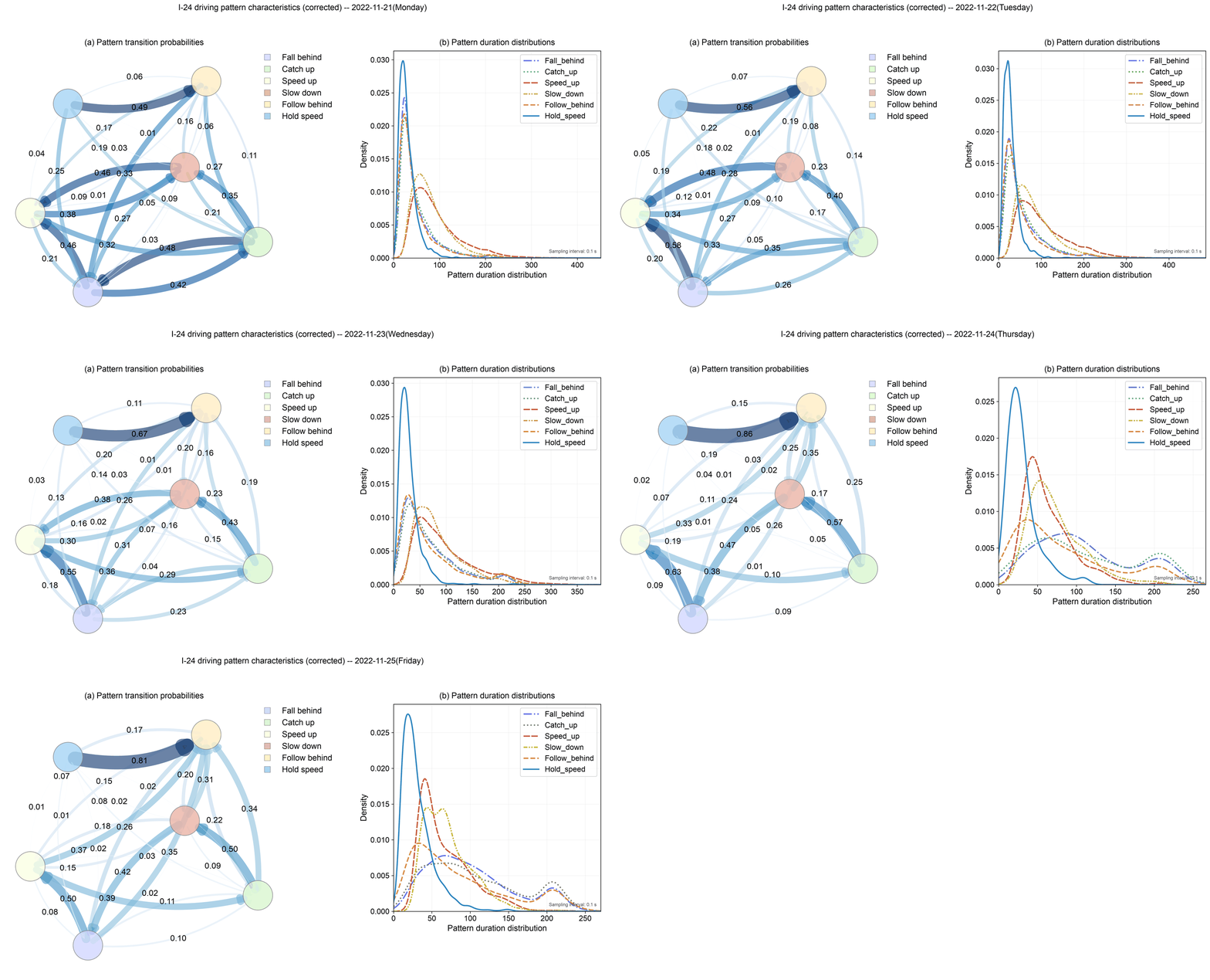
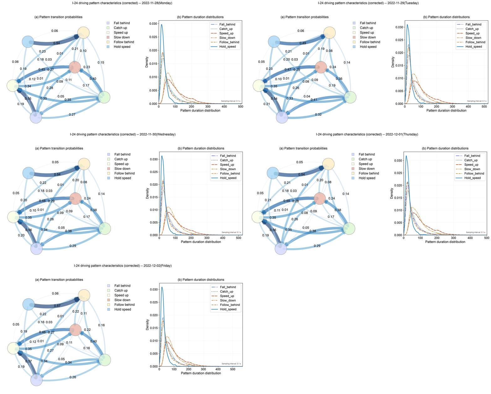
This dashboard explores the identification of driving patterns on a large-scale dataset using
the action-based framework developed by Yao et al. 2024. The framework labels car-following behavior into
six action patterns, helping to reveal traffic characteristics across different traffic conditions.
01
What the method does
Every car-following interaction is split into phases, each labeled as one of six action patterns based on
how the follower's speed, acceleration, and time headway to its leader change over time:
See Methodology for the full labeling process, thresholds, and a worked
example.
02
Why these ten days
The dataset used is the I‑24 MOTION INCEPTION dataset. The study window is two
consecutive work weeks on I‑24 near Nashville, TN: Week 1 (Mon Nov 21 –
Fri Nov 25, 2022) contains the Thanksgiving holiday on Thursday; Week 2
(Mon Nov 28 – Fri Dec 2) is an ordinary work week. A coherent, mechanistically
explicable holiday signature in Week 1 is itself a useful check: it shows the framework tracking a
real, independently known change in traffic conditions rather than behaving unpredictably.
Open Results to select any single day, compare two days, or compare the two
full weeks against each other.
Reproducible workflow
From trajectories to driving patterns
The method is carried over unchanged in its core logic from the earlier Lyft Level 5
study, with three corrections introduced since: speed restored as the top-priority signal, same-label
phases always consolidated, and a headway-refined relabeling pass added.
Concept overview
How a driving pattern is assigned
Driving variables
For each car-following pair: the ego (follower) vehicle's speed and acceleration, and its time
headway and speed difference to the leading vehicle (Yao et al. 2024).
→
Action trends
Between turning points, each variable is Increasing, Decreasing, or Steady.
→
Action phase
A segment over which every variable holds one trend at once.
→
Action pattern
Labeled Action phases that share a consistent driver response to traffic conditions, each
carrying a duration.
The six action patterns: Speed_up, Slow_down,
Catch_up, Fall_behind, Follow_behind, and
Hold_speed — assigned by the rule-based cascade in steps 01–06 below.
01
Three tracked signals
Follower speed v, follower acceleration a, and time headway τ to the
leader are each tracked throughout a car-following interaction.
02
Turning points
Local minima/maxima in each signal are candidate turning points. A candidate is discarded — its two
neighboring intervals merged — when the interval to it is both short (≤ the merge window) and low
amplitude, suppressing noise while preserving genuine trend changes.
03
State classification
Between consecutive retained turning points, each signal is Increasing, Decreasing, or steady (K),
compared against its own threshold (see Data & setup for exact values).
04
Speed-first labeling
Priority order, highest first: speed (Speed_up / Slow_down) → time
headway, only if speed is steady (Catch_up / Fall_behind) → acceleration,
only if speed and headway are both steady (Follow_behind, else Hold_speed). Reading the trend of each
signal over a phase — Increasing (I), Decreasing (D), or Steady (S) — against this order gives
the pattern label directly:
Signal
Speed_up
Slow_down
Catch_up
Fall_behind
Follow_behind
Hold_speed
Speed v
I
D
S
S
S
S
Time headway τ
–
–
D
I
S
S
Acceleration a
–
–
–
–
I or D
S
I = increasing, D = decreasing, S = steady, – = not decisive for this pattern (a
higher-priority signal has already determined the label).
05
Consolidation
Adjacent same-label phases are merged, and any phase shorter than the minimum retained length is
absorbed into a neighbor. A phase can therefore never transition into a same-label phase — the transition
matrix diagonal is zero by construction.
06
Headway-refined relabeling
Within every Speed_up/Slow_down phase, an underlying label is computed with speed excluded from the
cascade. If that underlying label is a single pure category across the entire phase, the phase is
relabeled to it; if it's mixed, the phase keeps its speed-first label. The corrected sequence is
re-merged. Both the primary and the refined sequence are retained as parallel analyses — see the
Results refinement-audit panel.
07
Worked example
One follower, real I-24 MOTION trajectory
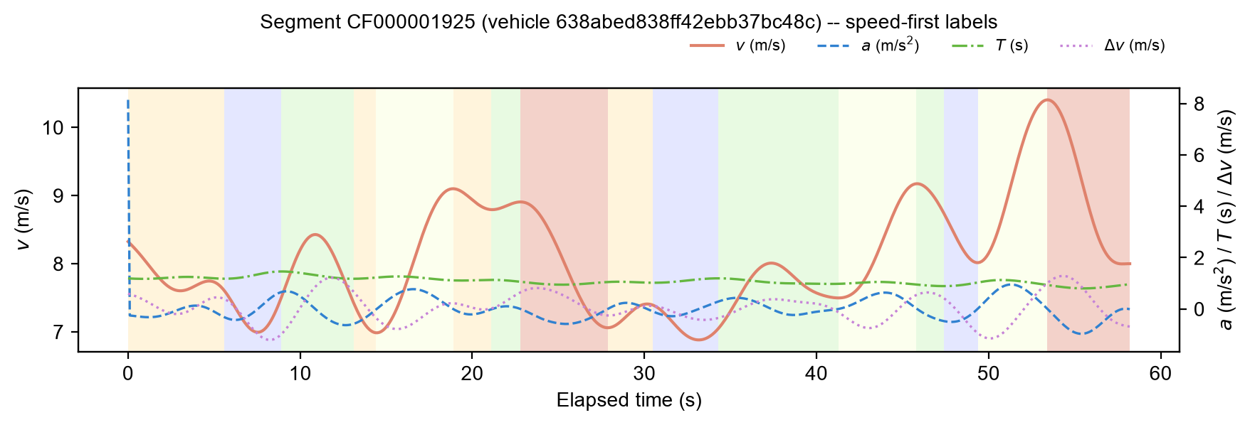
A real car-following segment from the study, with the four tracked variables plotted against elapsed time
and background shading showing the resulting Action pattern for each phase. Pick a different follower
vehicle to see how the same rule-based cascade plays out on a different trajectory:
Background color marks each phase's assigned pattern: lavender = Fall_behind, sage green =
Catch_up, salmon = Speed_up, pale yellow = Slow_down, tan = Follow_behind, light blue = Hold_speed (not
every pattern occurs in every segment). Vertical boundaries are the retained turning points from step 02.
Segments are drawn from the 2022‑11‑21 trajectory_examples output.
08
Statistics analysis
Once every phase in a day's traffic flow carries an Action pattern label, two complementary
quantities characterize the population: how likely a driver is to move from one pattern to another, and
how long each pattern tends to last.
Transition probabilities
Within a day's phase sequence (primary and headway-refined sequences are treated separately), let
ψ(Pi→Pj) be the observed count of transitions from pattern
Pi to pattern Pj. The transition probability is the row-normalized frequency:
Pr(Pn+1=Pj | Pn=Pi)=ψ(Pi→Pj)∑k=16 ψ(Pi→Pk)(1)
so each pattern's six outgoing probabilities sum to one. Because consolidation (step 05) forbids a phase
from following another of the same label, the diagonal Pr(Pn+1=Pi |
Pn=Pi) is zero by construction, for every pattern Pi.
Duration distributions
Rather than assuming a parametric form, each pattern's duration distribution is estimated
non‑parametrically. For pattern Pi, let {t1, …,
tz} be the durations, in seconds, of every retained phase labeled Pi on
that day. A Kernel Density Estimate (KDE) with a Gaussian kernel gives a smooth density
fi(t):
fi(t)=1zh∑j=1z Kt − tjh(2)
K(μ)=1√2πexp(−μ2 / 2)(3)
where z is the number of observed durations and h is the kernel bandwidth. Four
moments of the fitted density then summarize pattern Pi's duration characteristics — mean
μ (typical duration), variance σ2 (spread), skewness
γ1 (asymmetry), and kurtosis γ2 (tail weight):
μ=∫ t fi(t) dt
σ2=∫ (t−μ)2 fi(t) dt
γ1=∫ (t−μ)3 fi(t) dtσ3
γ2=∫ (t−μ)4 fi(t) dtσ4− 3(4)
This mirrors the distribution-based duration knowledge used to characterize Action patterns
in Yao et al. 2024.
Day-to-day transition change (L1 distance)
To quantify how much one day's transition structure differs from another's, let A and
B be the two days' 6×6 row-normalized transition matrices from Equation 1. The L1
(Manhattan) distance sums the absolute difference over every entry:
L1(A, B)=∑i=16 ∑j=16 |Aij − Bij|(5)
summed over all 36 ordered pattern pairs (i, j). L1(A, B) = 0 only
when the two days share identical transition probabilities for every pattern pair; since each row of
A and B sums to 1, the theoretical maximum is 12 (each of the six rows contributing
at most 2 to the sum). A small L1 distance between two days is therefore direct, interpretable evidence
that the underlying car-following behaviour was stable across them, while a large one flags a day whose
drivers moved between patterns in a measurably different way.
Experimental setup
I‑24 MOTION dataset and processing pipeline
Every numeric threshold below is reused unchanged from the original Lyft5 study, except the
segment-selection criteria that any new trajectory source necessarily requires.
01
Dataset
Vehicle trajectories reconstructed from a fixed camera network along a multi-mile section of
Interstate 24 near Nashville, TN. Each record gives back-center longitudinal and lateral position
(feet) and vehicle length; speed, acceleration, and lane are all derived during preprocessing. Data are
released as one file per calendar day, each on the order of 105–106
trajectories and tens of gigabytes.
This study uses ten weekdays: 2022-11-21 through 2022-12-02, split into Week 1 (with the
Thanksgiving holiday) and Week 2 (ordinary).
Raw file size and the daily camera-network collection window vary day to day, and matter for
interpreting the Results tab: most days cover a 4‑hour window, but Friday 11/25 was collected over
11 hours — nearly three times as long — so its raw scale is not directly comparable to an
ordinary day.
Day
Raw data size
Collection window
Segments extracted
Mon 11/21
20.13 GB
4 h
75,474
Tue 11/22
17.84 GB
4 h
63,409
Wed 11/23
12.98 GB
4 h
22,992
Thu 11/24 (Thanksgiving)
4.91 GB
4 h
1,421
Fri 11/25
25.78 GB
11 h
15,810
Mon 11/28
17.41 GB
4 h
65,149
Tue 11/29
20.00 GB
4 h
79,510
Wed 11/30
19.49 GB
4 h
83,242
Thu 12/01
19.53 GB
4 h
82,935
Fri 12/02
16.60 GB
4 h
60,446
"Segments extracted" counts an earlier candidate-segment pipeline stage, logged per day
before the retention criteria in step 03 are applied — it is not the same count as the final
retained car-following segments used elsewhere in this dashboard. Friday 11/25 collected for almost three
times as long as an ordinary day, yet still recorded barely a quarter of the segments seen on the
following week's ordinary Friday (12/02) — so the holiday-week effect visible in the Results tab
extends into Friday as well, not just Thanksgiving Thursday itself.
02
Preprocessing and smoothing
Each day's raw JSON is streamed record-by-record rather than loaded into memory. Position is smoothed
with a 0.6 s centered moving average, resampled to a fixed 0.1 s grid, and differentiated by
central difference for speed and acceleration. Lateral position is matched to lane-center offsets
(±5.5 ft tolerance) for lane assignment, and the nearest same-lane vehicle ahead is identified
as leader at every instant.
Continuity is enforced during segment extraction: consecutive samples from the same
follower–leader–lane combination remain part of one car-following segment only if the gap
between them is ≤ 0.25 s; a larger gap, or a change of leader or lane, closes the current segment
and starts a new one from the next sample. No interpolation is performed across a gap — small gaps
are simply tolerated within a segment, they are not filled in.
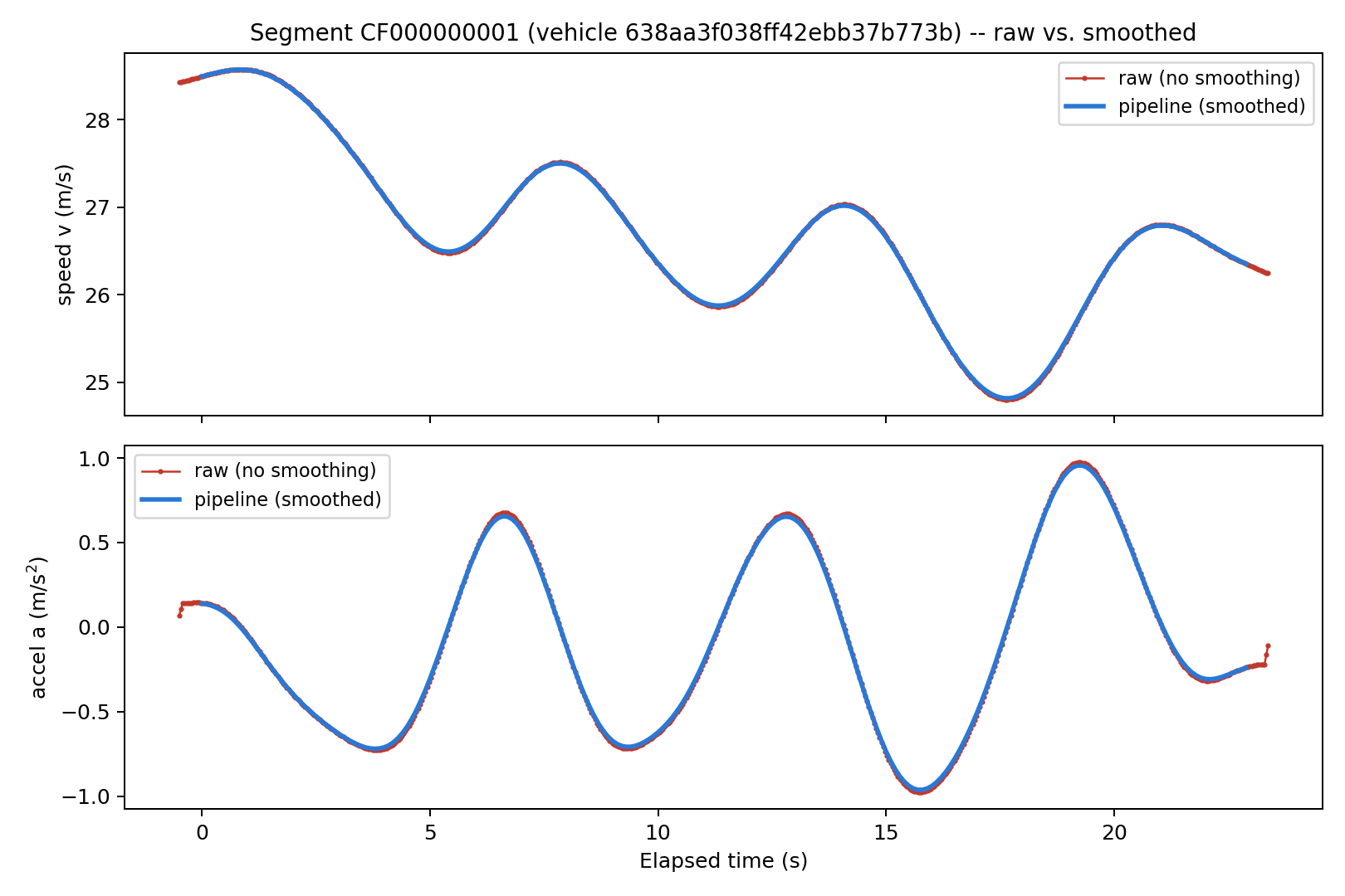
A direct comparison against unsmoothed raw positions found a maximum difference of 0.016 m/s in
speed and 0.024 m/s² in acceleration — one to two orders of magnitude below the pattern
thresholds below — indicating the smoothing step is a small safety margin, not a shaping filter.
Raw (red) vs. pipeline-smoothed (blue) speed and acceleration for one example segment — the
curves are visually indistinguishable, matching the maximum differences reported above.
03
Car-following segment retention criteria
Criterion
Threshold
Follower speed
v ≥ 3.0 m/s
Segment duration
≥ 20 s
Leader and lane
identical leader vehicle and lane throughout
Net space gap
0 < g ≤ 120 m
Time headway
τ ≤ 6.0 s
Sampling continuity
no gap exceeding 0.25 s
Kinematic plausibility
|v| ≤ 70 m/s, |a| ≤ 15 m/s²
04
Turning-point and state-classification thresholds
Signal
Change threshold
Symbol
Follower speed
1.5 m/s
θv
Follower acceleration
0.25 m/s²
θa
Time headway
0.15 s
θτ
Turning-point merge window
20 samples (2.0 s)
γ
Minimum retained phase length
10 samples (1.0 s)
Lmin
Identical to the Lyft5 study's thresholds, so any differences observed between the two
datasets' results reflect differences in the underlying traffic, not a re-tuning of the method.
Ten-day study results
How driving patterns shift across weeks
Two ways to explore the same ten-day study: compare Week 1 (Nov 21–25,
containing the Thanksgiving holiday) against Week 2 (Nov 28–Dec 2, an ordinary work
week) end to end, or drop into any single day's own pattern-recognition and pattern-characteristics
figures. Both views point to the same result: a large, short-lived shift exactly on the low-traffic
Thanksgiving Thursday, and an otherwise flat, stable signal.
Overview
Week 1 vs. Week 2 at a glance
Each animation steps day by day through its week, redrawing the same panel five times in a row. Watch
how Week 1 swings through the Thanksgiving trough while Week 2 barely moves — the
sections below break down exactly why, and the Day breakdown tab above shows every one of these frames
as its own static figure.
How often each pattern occurs, and how much that changes day to day
Both weeks, all ten days, side by side.
01
Statistics of driving patterns
Segments extracted per day, log scale
Retained volume, not phase composition — this is the raw scale of car-following
activity each day supplied to the pipeline before any pattern labelling happens.
02
Day-to-day transition change
L1 distance between consecutive days
Transition-matrix L1 distance (Equation 5, see Methodology)
between each day and the one before it, both weeks.
Findings
What the pattern breakdown shows
Week 1's transition-matrix distance spikes to 2.46 on Wed→Thu (Thanksgiving) — more
than double any other step that week, and roughly twenty times Week 2's Wed→Thu step
(0.12).
Week 2 stays flat all week: pattern-to-pattern switching behavior barely moves, holiday or
not — every one of its day-to-day steps stays under 0.6.
The spike lines up exactly with the volume collapse in the Statistics chart above (75,474
→ 1,421 segments by Thursday) — the sequencing shift isn't random, it tracks the traffic
drop day for day.
The spike is short-lived: by Thu→Fri the distance is back down to 1.06, close to the week's
own Mon→Tue baseline (1.06) — a one-day disruption, not a drift.
Pattern duration breakdown
How long each pattern lasts, and how that changes day to day
03
Duration trends by weekday
Mean phase duration, Mon–Fri
One subplot per pattern, each on its own y-scale. Catch_up, Fall_behind and Follow_behind
all climb steadily through Week 1 toward Thursday–Friday while Speed_up and Slow_down fall;
Hold_speed barely moves. Week 2 stays close to flat on every pattern.
Findings
What the duration breakdown shows
Week 1's pattern durations follow the same holiday signature as their sequencing. From Monday
to Thanksgiving Thursday, the three gap-adjustment patterns that don't involve an actual speed change
— Catch_up, Fall_behind, and Follow_behind — all lengthen sharply (Catch_up's mean
duration more than doubles, from 5.0 s to 11.0 s).
Speed_up and Slow_down — the two patterns driven by an actual speed change — shorten
over the same days (Speed_up: 9.3 s → 6.4 s). Hold_speed stays essentially flat
throughout, around 3.0 s on every day of both weeks.
Week 2 shows none of this movement: every pattern's mean duration stays within roughly a
second of its week-long average, every day.
Lower traffic pressure during the holiday trough is the natural read: with fewer vehicles to react
to, drivers spend longer gradually closing or opening a gap (Catch_up / Fall_behind / Follow_behind)
and less time making the sharp, reactive speed adjustments (Speed_up / Slow_down) that denser traffic
provokes.
Synthesis
Why this happens, and what it means
Why it happens. Thanksgiving produced a real, large drop in through-traffic on I-24 (a
92% collapse in retained car-following segments from Wednesday to Thursday alone), and that volume
collapse alone explains both shifts above. With fewer vehicles interacting, the reactive maneuvers
driven by an actual speed change (Speed_up, Slow_down) become less frequent and shorter, while the
slower gap-adjustment behaviors (Catch_up, Fall_behind, Follow_behind) that don't require a speed
change become more common and longer. One underlying cause — lower traffic pressure —
produces both the transition-sequence spike and the duration shift.
What it shows about the framework. The same pipeline that flags the holiday shift
precisely on Thanksgiving Thursday stays essentially flat across five ordinary Week 2 days and
recovers immediately once traffic returns to normal on Friday. That combination — sensitive to a
real, independently known change in conditions, but stable and specific under ordinary conditions
— is the behavior expected of a method that tracks genuine driving behaviour rather than noise or
drift. That the I‑24 MOTION results reproduce the same pattern-based structure originally
validated on the Lyft Level 5 dataset also supports the method transferring cleanly from a
smaller, controlled dataset to a larger, real-world one.
Bottom line: the framework is sensitive to meaningful behavioural
change, stable under normal conditions, and transferable to large-scale real-world data.
Day breakdown
Any single day, in detail
Pick a day below — shift-click a second day to compare it side by side. Figures use the
headway-refined sequence.
01
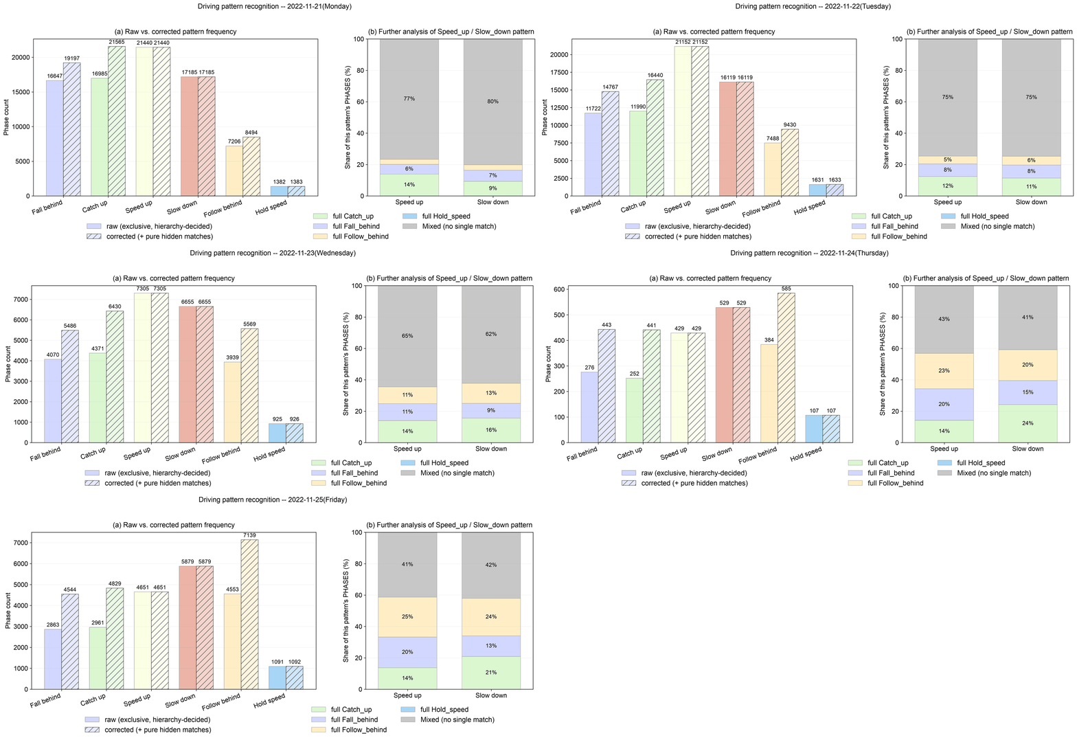
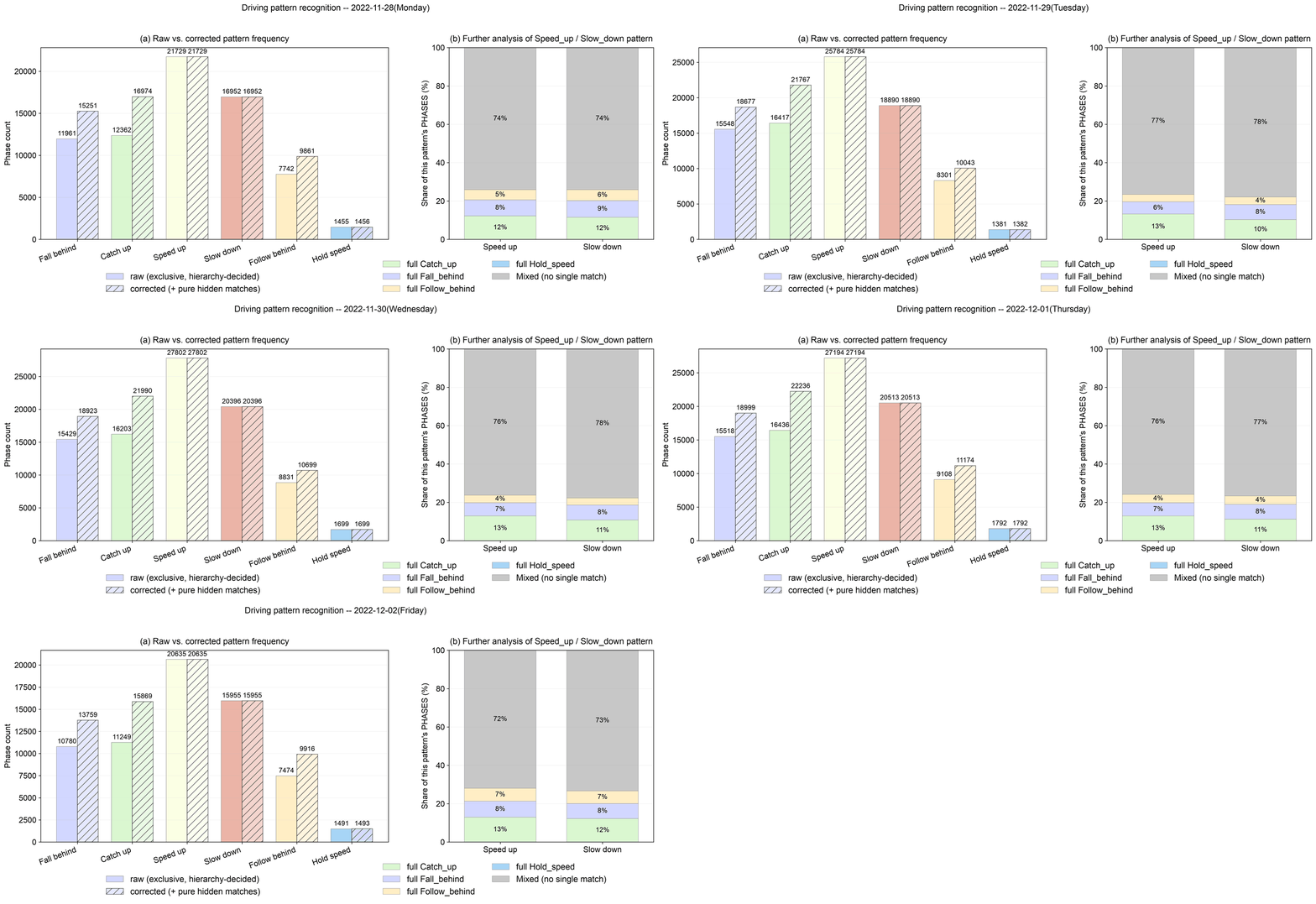
Pattern recognition
Raw vs. corrected pattern frequency, and further analysis of Speed_up / Slow_down
02
Pattern characteristics
Pattern transition probabilities and duration distributions (headway-refined)